Statistical Method for Automated Cell Detection and Counting
I used to work in a cancer lab at Lovelace Respiratory Reserach Institue where one of my jobs was to manually count cells under a microscope. We had thousands of microscope slides thousands of cells on each one. The entire process took ages. Sometimes you would lose track of which cells have alread counted and would have to start over. It's laborious, tedious projects such as these where automation by computers becomes extremely useful! During my time at LRRI I had heard of ImageJ and other such software that was suited for the task, however I was unfamiliar with their use and by the time I had gotten around to figuring it out we were on to the next project. Since then, I have been interested in attempting to write my own software that would be able to identify and count cells to be used in similar projects.
This notebook describes the methods I used to create a program for detecting and counting cells from a microscope image.
# Import necessary libraries
from IPython.display import Image
from IPython.display import Latex
import numpy as np
import cv2
import matplotlib.pyplot as plt
import matplotlib.cm as cm
from scipy import misc
from scipy import stats
import scipy.spatial.distance as dist
import PIL
from PIL import ImageDraw

plt.style.use("ggplot")
%matplotlib inline
Image/Data:
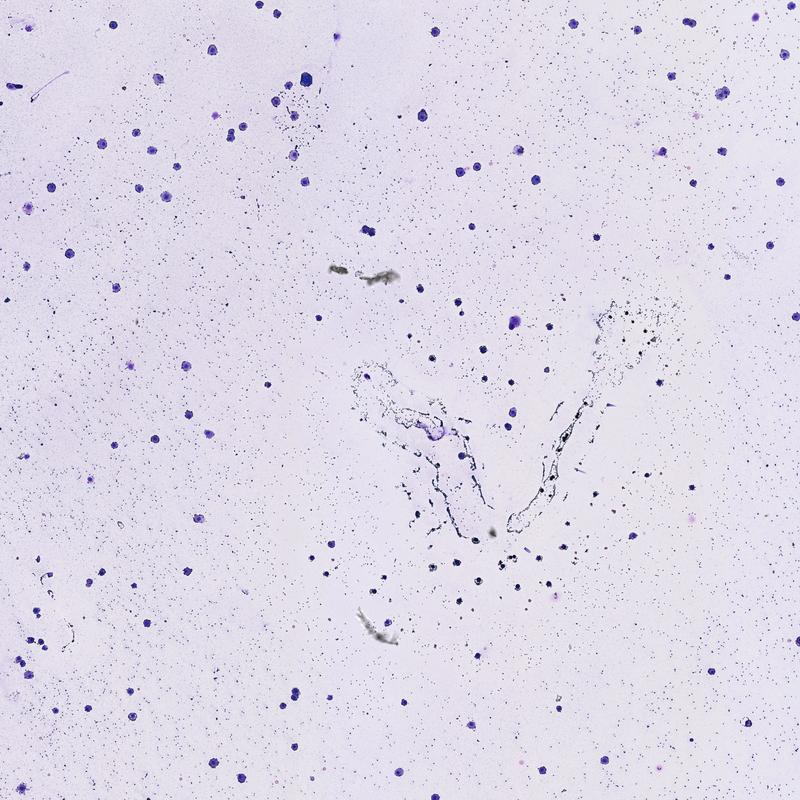
First, we will need to find an image with cells that we are intersted in counting. The figure below is a microscopy image of macrophages that have been stained purple. If you look closely you can see hundreds of smaller purple cells, these are bacteria. Right now we are only intersted in counting the larger macrophage cells.
Image(filename="A014 - 2014-03-05 11.47.59_x40_z0_i2j2.jpg")
Methods:
The entire process can be summarized in only a few steps
- Load image data
- Remove noise from the image
- Find cell locations
- Count cells
Loading image data:
Raw RGB pixel values are loaded into numpy array using the cv2 library.
file_path = "A014 - 2014-03-05 11.47.59_x40_z0_i2j2.jpg"
img = cv2.imread(file_path)
img.shape
Take the mean pixel value across each of the RGB channels. This will return a 8192 x 8192 dimensional matrix containing the mean value for each color.
img = np.mean(img, axis=2)
We now a have an 8192 x 8192 dimensional matrix to work with.
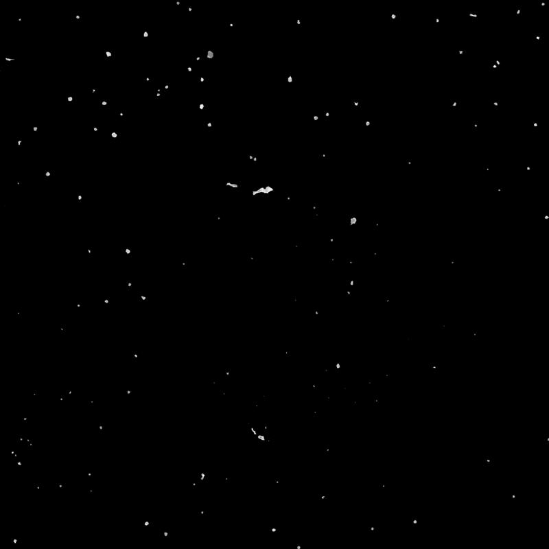
Removing noise:
We will create a function to facilitate noise removal. The function will apply dilation to remove background noise using the cv2 library then it will apply thresholding to remove any pixels that do not meet the thresholding requirement.
# Function for removing background noise
def remove_background_noise(img, dilations=1, kernel_size=5, thresh=200):
    kern = cv2.getStructuringElement(cv2.MORPH_ELLIPSE, (kernel_size, kernel_size))
    clean_image = cv2.dilate(img, kern, iterations=dilations)
    # Remove all pixels that are brighter than thresh
    return clean_image * (clean_image < thresh)
Now we can test it out. Lets create a clean image and print it to the screen.
# Create clean image
clean_image = remove_background_noise(img, dilations=2, kernel_size=20, thresh=200)
misc.imsave("clean_image.jpg", clean_image)
# Print image to screen
Image(filename="clean_image.jpg")
 "
>
"
>
Find Cell Locations:
To find cell locations we will need to scan through the cleaned image and find regions where pixels appear to be brighter than expected. As you can see in the image above, regions of high pixel intensity are cells. We can test to see if the pixel intensity within a certain region is bright than expected using a one sample t-test. With the t-test we wish to test the null hypothesis $H_{o}:\mu_{1} = \mu_{2}$ against the alternative hypothesis $H_{A}: \mu_{1} \ne \mu_{2}$ where $\mu_{1}$ is the mean pixel intensity for a given region $x,y$ and $\mu_{2}$ is the mean pixel intensity for the entire image (pixel population). We will use the significance level $\alpha=0.05$ which gives an allowable error of 5%. However, because we are making so many comparisons, we must use the Bonferroni adjustid significance level. This is determined by dividing the family error rate 0.05 by the total number of comparisons. The total number of comparisons depends on the step size from one window to the next. $$n = \frac{width}{step_{x}} \times \frac{height}{step_{y}}$$ With the image dimension above and a step size of 20 we can calculate the total number of comparisons as $$ n = \frac{8192}{20}\times\frac{8192}{20} = 167,772$$ The Bonferroni corrected $\alpha$ is calculated as $$\alpha = \frac{0.05}{167772} = 2.98x10^{-7}$$ We now have enough information to create our cell detection function.
# Function to detect cell locations using Bonferroni corrected one sample t-test
def detect_cell_location(clean_image, step_size=20, alpha=0.05, population_mean=220):
    n = clean_image.shape[1]
    m = clean_image.shape[0]
    x_coordinates = []
    y_coordinates = []
    number_of_comparisons = np.round((n/step_size)*(m/step_size))
    bonferroni_alpha = 0.05 / float(number_of_comparisons)
    for y in xrange(0, m, step_size):
        for x in xrange(0, n, step_size):
            wind = clean_image[y:y+step_size, x:x+step_size].flatten()
            t_statistic, p_value = stats.ttest_1samp(wind, population_mean)
            if p_value < bonferroni_alpha and t_statistic > 0:
                x_coordinates.append(x)
                y_coordinates.append(y)
    return (x_coordinates, y_coordinates)
Now lets run it to extract the x and y coordinates for each cell
# Determine the pixel population mean
pop_mean = np.mean(clean_image)

# Extract cell locations
x_coordinates, y_coordinates = detect_cell_location(clean_image, population_mean=pop_mean)
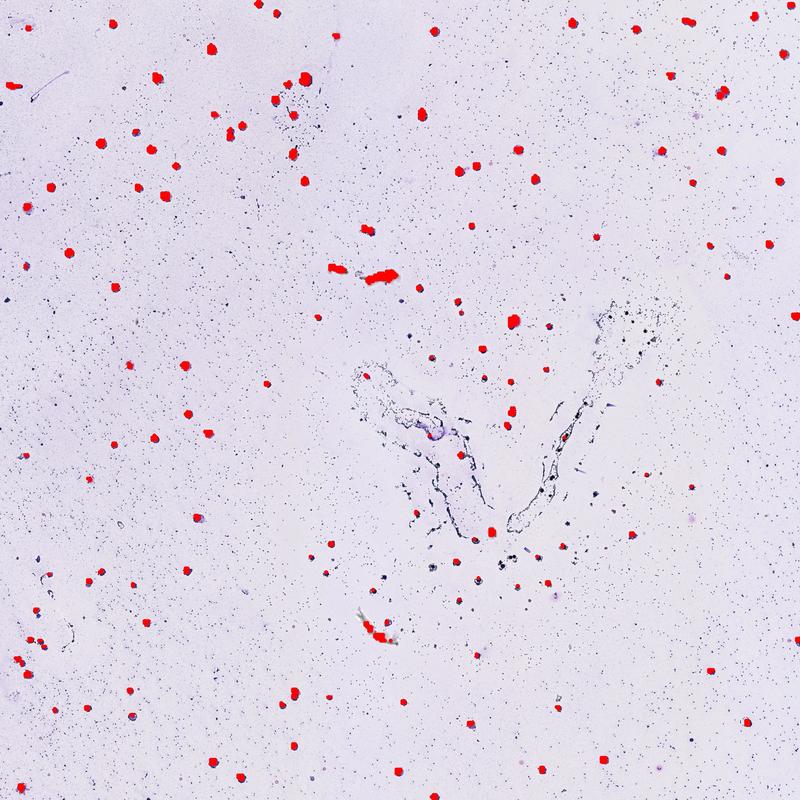
Now then, lets go ahead and overlay the coordinates on top of the original image to see how we did
# Function for overlaying points on image
def overlay_coordinates_on_image(image_path, x_vals, y_vals, point_radius=20):
    original_image = PIL.Image.open(image_path)
    draw = ImageDraw.Draw(original_image)
    for i in range(len(x_vals)):
        x = x_vals[i]
        y = y_vals[i]
        draw.ellipse((x-point_radius, y-point_radius, x+point_radius, y+point_radius), fill=(255,0,0))
    return original_image

labeled_image = overlay_coordinates_on_image(file_path, x_coordinates, y_coordinates)
labeled_image.save("original_with_points.jpg")
Image(filename="original_with_points.jpg")
 >
>
Count Cells:
Now it almost seems like we're finished, but if you were to zoom in on this image you would see that there are many points associated with each cell. In order to get an accurate cell count we need to group points that are close together into a single point called a centroid. After we merge all adjacent points, we can count the number of remaining centroids to get an official cell count.
In order to group the points we must first defined how close two points must be in order to be considered part of the same cell. If we were to zoom in on the image we would see that the diameter of each macrophage is about 60 pixels. Therefore, the maximum distance two points can be while still being associated with the same cell is about 60 pixels. We can now write a function to group points that are < 60 pixels away from one another. In the function below, when two points are merged a centroid is created with an x-coordinate of $x = \frac{x_{1} + x_{2}}{2}$ and a y-coordinate of $y = \frac{y_{1} + y_{2}}{2}$
Non-weighted clustering:
# Function to perform non-weight based clustering on points
def cluster_points(x_vals, y_vals, max_distance=60):
    xy_points = [[x_vals[i], y_vals[i], 0] for i in range(len(x_vals))]
    new_length = len(xy_points)
    old_length = 0
    while new_length != old_length:
        old_length = len(xy_points)
        for i in range(len(xy_points)):
          for j in range(i+1, len(xy_points)):
                try:
                  dist_between_points = dist.euclidean(np.array(xy_points[i][:2]), np.array(xy_points[j][:2]))
                  if dist_between_points < max_distance:
                      new_x = (xy_points[i][0] + xy_points[j][0]) / 2.0
                      new_y = (xy_points[i][1] + xy_points[j][1]) / 2.0
                      xy_points[i][0] = new_x
                      xy_points[i][1] = new_y
                      xy_points[i][2] += 1
                      del xy_points[j]
                      new_length = len(xy_points)
                except:
                    pass
    x_vals = [i[0] for i in xy_points]
    y_vals = [i[1] for i in xy_points]
    num_points_found = [i[2] for i in xy_points]
    return (x_vals, y_vals, num_points_found)
Now lets cluster all the points we found in the previous step to get a cell count
# Cluster points into centroids using the non-weight based method
cells_x, cells_y, num_points_found = cluster_points(x_coordinates, y_coordinates)
print "Found %d cells!" % len(cells_x)
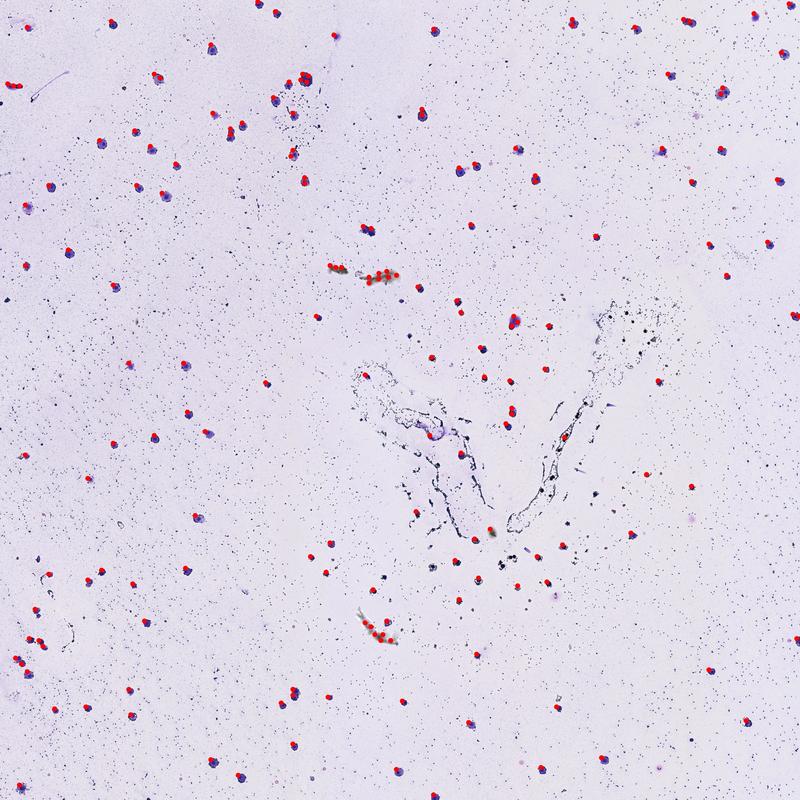
Now that we've reduced all our points down to clusters let's plot the cluster centroids to identify the locations of our cells
# Overlay centroid locations
cell_count_overlay = overlay_coordinates_on_image(file_path, cells_x, cells_y, point_radius=25)
cell_count_overlay.save("cell_count_overlay.jpg")
Image(filename="cell_count_overlay.jpg")
 "
>
"
>
Weighted clustering:
From the image above, you can see that we've done a pretty good job identifying cell locations in the image. One noticable issue is that cells that are close together have only one label and thus, have only been counted once. One possible solution is to weight each point's influence over the centroid's location based on how far it is away from the current centroid position. Using this method, a point that is far from the centroid's has less influence on the final centroid location.
# Function used to weight pixel influence on centroid
def weight_function(dist, p=1):
    return 1 / float(np.power(1 + dist, p))

# Cluster points using distance-based weighting
def cluster_points_weighted_distance(x_vals, y_vals, p=1, min_distance=60):
    xy_points = [[x_vals[i], y_vals[i], 0] for i in range(len(x_vals))]
    new_length = len(xy_points)
    old_length = 0
    while new_length != old_length:
        old_length = len(xy_points)
        for i in range(len(xy_points)):
            for j in range(i+1, len(xy_points)):
                try:
                    dist_between_points = dist.euclidean(np.array(xy_points[i][:2]), np.array(xy_points[j][:2]))
                    #if dist_between_points < min_distance:
                    weighted_distance = weight_function(dist_between_points, p=p)
                    new_x = xy_points[i][0] + weighted_distance * (xy_points[i][0] - xy_points[j][0]) / 2.0
                    new_y = xy_points[i][1] + weighted_distance * (xy_points[i][1] - xy_points[j][1]) / 2.0
                    xy_points[i][0] = new_x
                    xy_points[i][1] = new_y
                    xy_points[i][2] += 1
                    if dist_between_points < min_distance:
                        del xy_points[j]
                    new_length = len(xy_points)
                except:
                  pass
    x_vals = [i[0] for i in xy_points]
    y_vals = [i[1] for i in xy_points]
    num_points_found = [i[2] for i in xy_points]
    return (x_vals, y_vals, num_points_found)
Now let's see it in action
# Find new cluster locations using distance-based weighting
cells_weighted_x, cells_weighted_y, num_points_found = cluster_points_weighted_distance(x_coordinates, y_coordinates, p=2)
print "Found %d cells!" % len(cells_weighted_x)
# Overlay centroid locations
weighted_cell_count_overaly = overlay_coordinates_on_image(file_path, cells_weighted_x, cells_weighted_y, point_radius=25)
weighted_cell_count_overaly.save("weighted_cell_count_overlay.jpg")
Image(filename="weighted_cell_count_overlay.jpg")
 "
>
"
>
Gravitational clustering:
Okay great, this works but fails to take into account how may points have been averaged in to the current centroids location. A better method would be to use a gravity analogy. For example, if a centroid has been created from the merger of 15 points, we can think of this as having a mass of 15. Now if another single point (with a mass of 1) acts on this centroid (mass of 15) it would not make sense for it to have a substantial influence on the final position of the centroid. Both masses are experiencing the same force, however the more massive of the two objects has more inertia and therfore its position would change less than the less massive object's position. Consider the force experienced between two particles as determined by the gravity formula below: $$F_{g} = G\times\frac{m_{1}m_{2}}{d^2}$$
# Function to calculate the force experienced by two masses
def gravitational_force(dist, m1, m2, G=1):
    return G*(m1*m2)/float((np.power(dist,2)))

# Cluster points based on gravitational attraction
def gravity_based_clustering(x_vals, y_vals, G=1, min_distance=60):
    # Start each point off with a mass of 1
    xy_points = [[x_vals[i], y_vals[i], 1] for i in range(len(x_vals))]
    new_length = len(xy_points)
    old_length = 0
    while new_length != old_length:
        old_length = len(xy_points)
        for i in range(len(xy_points)):
            for j in range(i+1, len(xy_points)):
                try:
                    dist_between_points = dist.euclidean(np.array(xy_points[i][:2]), np.array(xy_points[j][:2]))
                    m1 = xy_points[i][2]
                    m2 = xy_points[j][2]
                    force = gravitational_force(dist_between_points, m1, m2, G=G)
                    acceleration = force / float(m1) # Distance centroid moves
                    new_x = xy_points[i][0] + acceleration * dist_between_points
                    new_y = xy_points[i][1] + acceleration * dist_between_points
                    xy_points[i][0] = new_x
                    xy_points[i][1] = new_y
                    xy_points[i][2] += 1
                    if dist_between_points < min_distance:
                        del xy_points[j]
                    new_length = len(xy_points)
                except:
                  pass
    x_vals = [i[0] for i in xy_points]
    y_vals = [i[1] for i in xy_points]
    num_points_found = [i[2] for i in xy_points]
    return (x_vals, y_vals, num_points_found)
# Find new cluster locations based on gravitational attraction
cells_gravity_x, cells_gravity_y, cell_masses = gravity_based_clustering(x_coordinates, y_coordinates, G=0.001, min_distance=60)
print "Found %d cells!" % len(cells_gravity_x)
gravity_cell_count_overaly = overlay_coordinates_on_image(file_path, cells_gravity_x, cells_gravity_y, point_radius=25)
gravity_cell_count_overaly.save("gravity_cell_count_overlay.jpg")
Image(filename="gravity_cell_count_overlay.jpg")
 "
>
"
>
Conclusion:
Comparing the various methods above you can see we get slightly different cell counts. After looking at the labeled images, it seems that the weight based methods provide better results when two cells are close together. Of course there are many hyperparameters that can be adjusted which may result in better or worse performance. Also, there appears to be several false positives resulting from residual noise that remained in the images after the cleaning step. However, depening on the quality of the input image and the amount of time spent tweeking parameters, it may be possible to improve accuracy further.
Future Direction:
This notebook provided a statistics based approach for detecing and counting cells in a microscopy image. Although effective, this method requires some amount of hard-coding and manual intervention/oversight. In a future project, I will use these methods to generate training data to be used in training of machine learning algorithms/classifiers for more robust/automated methods of cell detection.